May 30, 2017
DCE MRI Accuracy Research
A visualization of 4D DCE-MRI volume with a bolus injection in a patient with glioblastoma. Data from public dataset, gif by me.
In non-scientific terms, this means that patients are injected with a fluid ("contrast agent") that shows up brightly on MRI scans specifically where their tumor is. The speed with which this contrast agent seeps into a tumor, and then seeps out, might tell us something about how deadly or treatable that tumor is. To study this better, we take what is essentially a 3D video of someone's brain while they are being injected. This way, we can watch in real time how quickly that fluid is taken up.
When trying to understand contrast agent flow in DCE-MRI, radiologists focus on the variables ktrans and Ve. These variables represent proxies for membrane permeability and extracellular space, respectively. Within tumors, the magnitude of these values has some correlation with patient prognosis, so they have been deemed important to measure. One acquires these variables by fitting the pixel-wise (technically, "voxel"-wise) time curves found in 4D DCE-MRI volumes using a well-known model called the Tofts model. Each voxel in 3D space will thus have one ktrans and one ve associated with it, creating 3D ktrans and ve "maps" from the original 4D DCE-MRI.
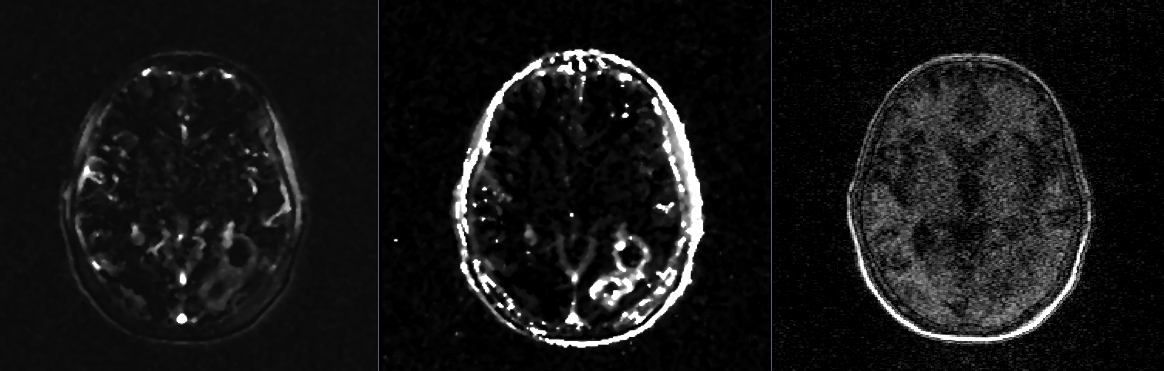
From left to right: one slice of a ktrans map, a ve map, and the first time point of a DCE-MRI.
Problem solved? Not quite. Our software performed well because of certain de-noising features it included when analyzing time-curve signals. It was thus very accurate on the digital phantoms referenced in the previous paper, which had an extremely regular spatial structure that is easy to denoise. Patient data has a very heterogenous spatial structure that is probably harder to accurately denoise than the digital phantom. So, my algorithm would probably perform worse on patient data, and maybe even worse than some of the algorithms it was tested against in the paper referenced above.
To address this problem, I took an existing public dataset of patients with glioblastoma and DCE-MRI scans, and created "digital patient phantoms". These are phantom DCE-MRIs where ktrans and ve values are known, but are arranged in the exact same spatial structure that one would expect in a patient. I generated these by generating ktrans and ve maps from the original raw patient datasets, and then integrating them back into "ideal" 4D volumes for which the original ktrans and ve maps would by definition be ground-truth. These maps would look like the original patients, but be totally absent of noise. Because we know their ground truth values, they can then be used to evaluate the performance of different ktrans/ve fitting softwares. A conference paper detailing these phantoms was accepted to SPIE 2017, and a Dropbox folder with the phantoms can be found here.
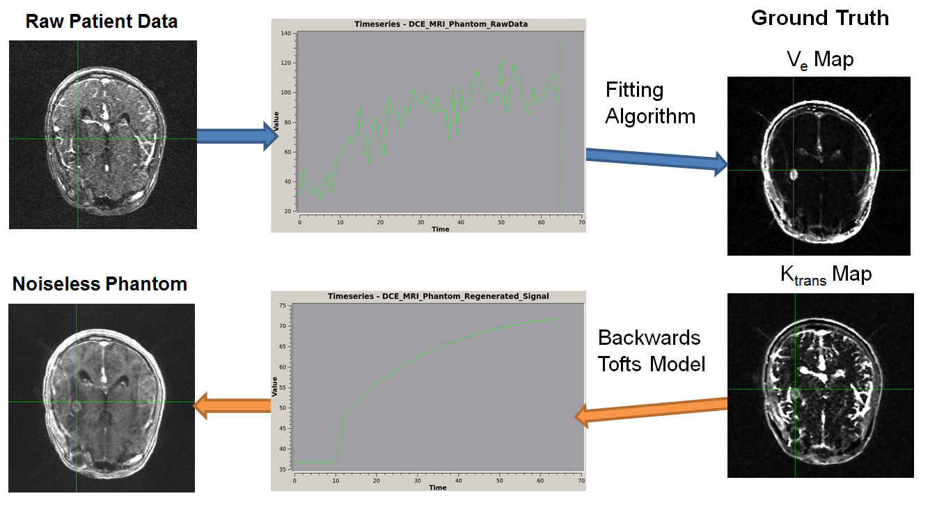
A figure from our recent accepted abstract at SPIE 2018. It represents a schematic for the creation of the QTIM/RIDER Anatomical Phantoms. 3D Ktrans and Ve Parameter Maps are generated from 4D DCE-MRI images from a patient with glioma. Those maps are used to create idealized, noiseless versions of the original input time-intensity curves. An anatomical 4D DCE-MRI results with the original parameter maps as ground-truth.